
We Simulated the Mariners’ Playoff Lineup, and It Wasn’t Even Close to Optimal (Part 1)

Dan Wilson (Photo by Steph Chambers/Getty Images); Dominic Canzone (Photo by Steph Chambers/Getty Images); Jorge Polanco (Photo by Steph Chambers/Getty Images)
Imagine this: With a simple lineup simulation and optimization model, the Mariners might have won the World Series.
Data scientist and Mariners fanatic Luisarturo Castellanos, based in Mexico, has developed a lineup simulation that calculates the ideal batting order. According to his model, the Mariners’ playoff lineup against Toronto was not just less than ideal; it was nearly half a run worse per game on average.
In the decisive game against the Blue Jays, Dan Wilson’s lineup was projected to score 4.43 runs per game, while the optimal simulated lineup would have averaged 4.90 runs. That may sound small, but over a series or full season, the difference adds up.
Please note that this article goes through the optimal lineup based on a typical game. We plan to re-do the simulation in a later research paper that takes into account pitcher splits and home/away splits.
The Mariners’ final postseason lineup looked like this:
Julio Rodríguez – CF
Cal Raleigh – C
Josh Naylor – 1B
Jorge Polanco – DH
Randy Arozarena – LF
Eugenio Suárez – 3B
J.P. Crawford – SS
Leo Rivas – 2B
Victor Robles – RF
While this group is loaded with talent, the order raises questions about efficiency and run production.
If the Mariners had used the optimal lineup for every game this season, the team would have scored an estimated 76 more runs. Using the rule of thumb that 10 runs equal one additional win, that translates to roughly eight extra victories across the year. In other words, an optimized lineup could have increased their chance of winning each game by about five percent.
Baseball is unique in that all nine players must bat, meaning even average hitters can find themselves in critical situations. Over 162 games, those moments accumulate, creating the perfect dataset for modeling.
With modern tools such as @Risk, analysts can build stochastic models that go beyond traditional heuristics to simulate expected outcomes for every possible lineup combination. The result is a statistically informed blueprint for maximizing run production and improving a team’s chances of postseason success.
Background
The goal of a baseball game is to score more runs than the opponent. Therefore, the team’s manager must decide the order at which players will come to bat during the game with the clear intention of maximizing the number of runs that his team can score during that game.
What makes baseball unique from other sports is that all 9 players that comprise the starting lineup have the same opportunities to contribute to score runs, because all players should take their turn to bat. Thus, sometimes the most critical at bat of the game might face a “random player” which might not necessarily be the best batter available.
The fact that a baseball season consists of 162 games provides a big sample in which many players end up with approximately 700 plate appearances. This big data is the basis to build a stochastic model that resembles what happens in a baseball game. Old board games like Strat-O-Matic used to mechanically simulate the different random outcomes of a baseball game, today, with the use of @Risk, an add-on that runs on Excel, we can build a stochastic model to optimize the lineup of a baseball team.
The Stochastic Model.
A baseball game is so complex yet so simple that it can be modelled assuming some restrictions. To begin with, the large sample size of stats available for each player provides a robust basis to build a probabilistic model, and even though the game is very complex, we can simplify it by considering only the 8 unique outcomes of each play which are:
1. Strikeout (generally when the batter didn’t put the ball in play and got the third strike either called, swinging, or by a foul tip).
2. Groundout (any out in which the ball hit the ground, but still an out was made).
3. Flyout (or a popout, or a lineout, i.e. any ball in play in which the ball was caught in the air).
4. Base on Balls (a plate appearance in which the batter reaches first base safely either by 4 balls (intentionally or unintentionally) or by a hit by pitch).
5. Single (a ball in play in which the batter reaches first base safely).
6. Double (a ball in play in which the batter reaches second base safely).
7. Triple (a ball in play in which the batter reaches third base safely).
8. Homerun (either an out the park or a inside the park touch em all).
The outcomes are color-coded so that we can easily identify those plays that are negative for the offense in red-orange codes, while the positive outcomes are the green-blue codes. Some assumptions most be made about this outcomes, which are the following: whenever a strikeout occurs, all baserunners (if any) stay put in their current bases; whenever a groundout occurs, all baserunners are able to move one base forward and the batter is the one who is out (although we know that sometimes the batter reaches base on a forced out and another runner might be the one who was out, we will simplify the model assuming this); whenever a flyout is recorded all runners stay put in their current bases, unless a runner is on third base and there are less than 2 outs, in which case, a sacrifice fly will occur and the runner at third base will score a run. For the positive outcomes, if a base on balls happens all forced runners will advance, otherwise they will stay put; for a single runners advance one base, a double moves runners 2 bases, a triple scores everyone but the batter; and finally, a homerun scores every runner including the batter.
The outcome of each play in a baseball game is unknown, but we can model the probability of each outcome based upon each player’s stats, thus modelling stochastically a whole baseball game from the perspective of the offense.
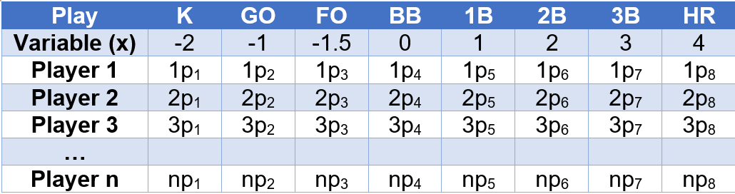
Parsimoniously a general discrete distribution is proposed to model the random variable of the outcome of one plate appearance of a particular player as follows:

Where pi >= 0 for every i, i.e. all probabilities most be non-negative and p1+p2+p3+p4+p5+p6+p7+p8=1, i.e. the sum of all probabilities most be equal to one. Calculating these probabilities becomes straightforward by simply dividing each stat by the total number of plate appearances a batter had, for instance:

Once the probabilities for each player have been calculated (p1, … p8) a parameter matrix is built as follows:
The Simulation and the Results
The chart below shows that Raleigh and Suárez are the players with highest HR probabilities (blue bars: 8.5% and 7.5% respectively, which makes sense since Raleigh hit 60 HR while Suárez hit 49 during the recent season), but Suárez is also the one with the highest K probability (dark red bars: 29.8%). On the other hand, Canzone and Naylor are the players with the best singles rate (light green bars: 19% and 18.2% respectively). Rivas walked at a 18.9% (dark green bars) rate which makes him an asset. An easy way to discriminate “good” players from “bad” ones is to see how high the orange bar goes, because this indicates the probability of being out. Garver, Robles and Suárez are the players with the highest probability of being out, reaching almost a 70% chance for those 3 players. Conversely, their probability of reaching base safely was the smallest one, roughly 30% (1-0.7).

The Optimal Lineup
The lineup that gives the Mariners the best chance to score as many runs as possible in the lineup below. It is far from traditional as it puts one of the top power hitters in the 8 spot. Dominic Canzone had a really strong season from a singles and OBP%, which is why the model puts him in the #1 spot. This lineup on average score 4.9 runs per game… much higher than the 4.4 runs per game from the lineup that we fielded during game 7 of the ALCS.

Results and explanation of Simulation
The RiskDiscrete function of @Risk is useful to model the phenomena, by using the code of each variable and @Risk’s function, =RiskDiscrete(x1:x8,p1:p8) will simulate a discrete value x upon the sample space (-2, -1.5, -1, 0, 1, 2, 3, 4) where each possible outcome has a different probability given by the p1..p8 for each player. Notice that the actual outcome of the variable x is completely meaningless, in the sense that the expected value of x doesn’t have any meaning, but it will be used as a code to simulate a whole baseball game. As an example, the following chart illustrates the distribution for Cal Raleigh, the Mariners catcher, using his 2025 stats:
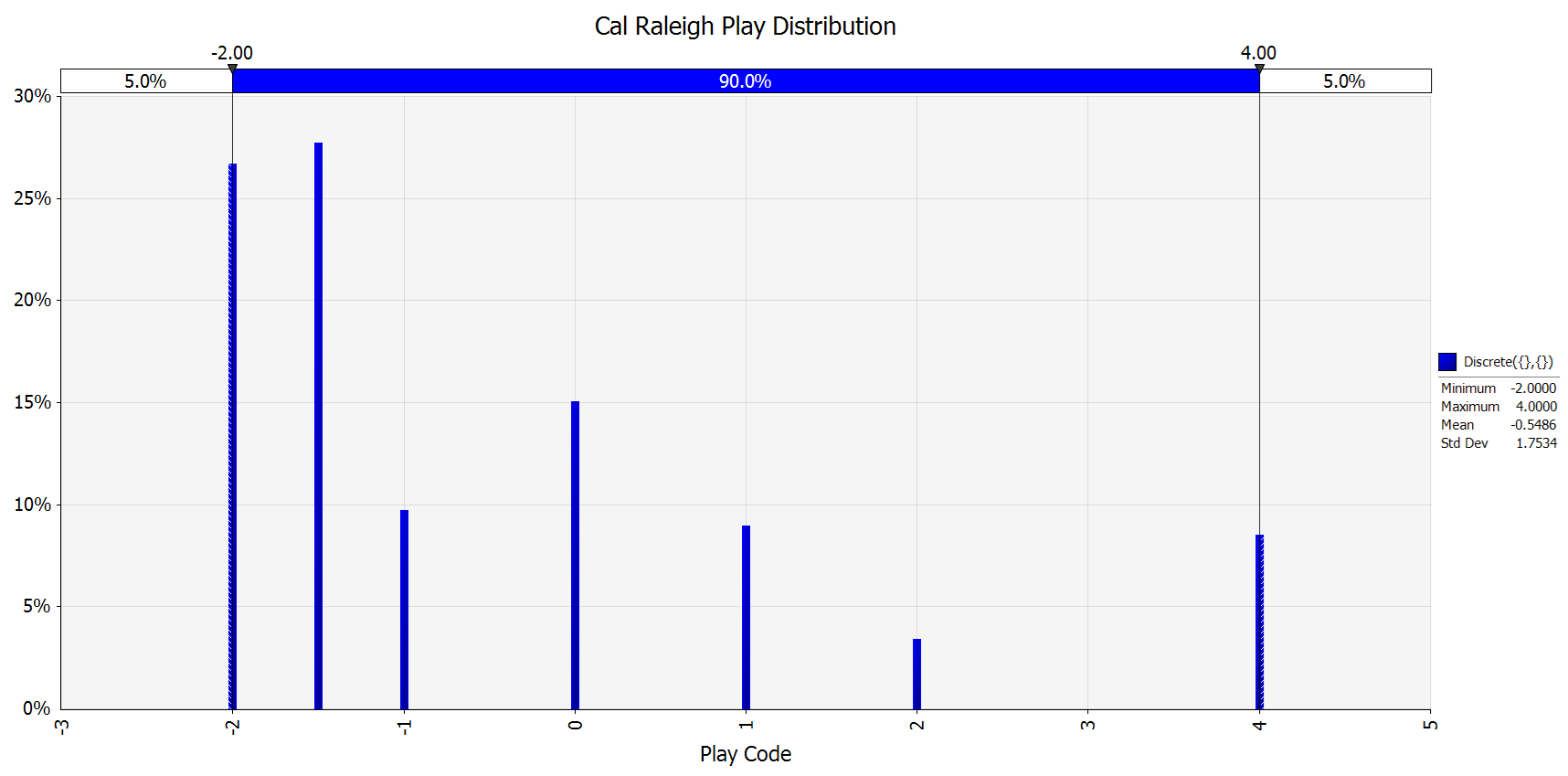
The chart shows that most likely outcome (the highest bar) is a flyout (-1.5 code) for Cal Raleigh, with a 27.7% probability (p3). The second most likely outcome is a strikeout (-2 code) with a 26.7% probability (p1). On the other hand, the most likely positive outcome for Raleigh is a walk (0 code) with 15% probability (p4), with the single and homerun closely similar with 8.9% and 8.5% probabilities respectively (p5 and p8). Obviously, the triple is the least likely outcome since seldom does Cal hit a triple.
However, the play codes don’t make any sense by themselves, for instance the mean value of x is -0.5486 which can’t be interpreted meaningfully. But the codes can be translated into simulating the evolution of a baseball game derived from the outcomes of each play.
To do this a worksheet was created where we take control of the bases and outs situation depending on each play’s outcome. The following chart illustrates the random process:
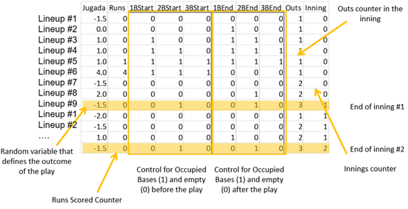
The figure above shows an example of a simulation of 2 innings as follows. The first column has the 9 players in sequence as the lineup is composed, with the #1 batter following the #9 every time after the 9th batter hits as usual in any baseball game. The second column (Jugada = play code) refers to the actual random variable for each play’s outcome. The third column (Runs) is the counter for how many runs are scored on each play. The next 3 columns (1BStart, 2BStart, and 3BStart) represent the bases occupied before the play, with a 0 code for empty and a 1 for occupied. The next 3 columns (1BEnd, 2BEnd, 3BEnd), represent the bases occupied after the play. The next to last column controls the number of outs, while the last column controls the inning.
So, in this example, the first player lead off the game with a Fly Out (play code = -1.5), so no bases were occupied, but the second player drew a walk (play code = 0), thus occupying first base after the play. Then, the third and fourth batters hit singles, thus loading the bases, while the fifth one, also hit a single, and that’s when the first run was scored (Runs=1). The sixth batter hit a homerun (play code = 4), scoring 4 more runs, and emptying the bases. The seventh batter was out on a Flyout (play code = -1.5) which was the second out of the inning. Batter #8 hit a double (play code = 2), and finally batter number 9 hit another fly out (play code = -1.5) to end the first inning.
The second inning starts with the leadoff hitter again this time striking out (play code = -2), the second batter was out on a flyout for out #2, and even though the third batter hit a single (play code = 1), he was left stranded because the cleanup hitter hit another flyout to end inning number 2. Notice that the bases are erased (all reset to 0) when a new inning starts.
This random process continues indefinitely, but runs are only accounted for until 9 innings are completed. This is another assumption the model makes, although it is known that sometimes the home team won’t need to bat in the 9th inning if the team is ahead, while other times extra-innings are needed if the game is tied, for the purpose of this model we always consider 9 full innings to simulate a whole baseball game. The model also assumes that the defense doesn’t make any errors, but also doesn’t make any double plays.
However, another important element of the baseball game and the lineup construction process deals with stolen bases. The model considers the possibility of a runner stealing a base. To stochastically model the stolen bases, we used 3 additional variables for each player:
1. Stolen Bases (SB)
2. Caught Stealing (CS)
3. Stolen Bases Opportunities (SBO).
Based upon these statistics, 2 parameters were estimated for each player, which are:
this refers to the propensity of stealing bases, in other words, how often does a player try to steal a base, and:
this refers to the efficiency at stealing bases, i.e. the proportion of steal attempts that are successful.
Once the parameters are estimated for each player, 2 different random variables are simulated using Bernoulli distributions.
1. Bernoulli (SBprop), for whether the player will attempt a steal
2. Bernoulli (SBeff), to determine whether the steal attempt was successful or not.
Hence, the model has 2 control cells to consider the stealing process, before the outcome of each play, as follows: if there is a runner on first base and there is no runner on second base, and if the Bernoulli variable for trying a steal is equal to 1, then a steal attempt is considered. Finally, if the Bernoulli for success is equal to 1, then the runner at first base is moved into second base before the next play (successful steal, SB), but if this variable is = 0 then the runner is erased and an additional out is added (caught stealing, CS).
A baseball game usually lasts for 9 innings, that is why the process continues indefinitely until the innings counter reaches 9. The minimum number of total plate appearances is 27 (3 outs x 9 innings), but there is no upper limit (maximum) number of plate appearances, rather, players will keep batting as many times as necessary to generate 27 outs.
The output variable (=RiskOutput) will be the sum of the runs scored for the whole 9 innings. A cell was created in the worksheet that sums all runs scored in the process up to the moment in which 9 innings are reached and this cell is defined as an output variable in @Risk so that its outcome is recorded after each iteration in the Monte Carlo simulation.
Application of the Model
The model needs at least 9 different players, each with his own parameters for the Discrete Distribution. A team with only 9 players can build a different lineup in 9! different ways, i.e. there are 362,880 different possible lineup combinations, but as the number of bench players increases the number of lineup combinations also increases significantly. For instance, if 2 bench players are added, then 11! = 39’916,800 different lineup combinations could be penciled, which is 110 times more combinations than with only 9 players.
As an example of the application of the model, the 11 players that were playing regularly in the recent 2025 ALCS by the Seattle Mariners lineup will be used, these were in order of position played: 1. Raleigh, 2. Naylor, 3. Polanco, 4. Crawford, 5. Suárez, 6. Arozarena, 7. Rodríguez, 8. Robles, 9. Canzone, 10. Garver, 11. Rivas. The following chart summarizes the probabilities for each player using the same color-coding for each play’s outcome:

The chart shows that Raleigh and Suárez are the players with highest HR probabilities (blue bars: 8.5% and 7.5% respectively, which makes sense since Raleigh hit 60 HR while Suárez hit 49 during the recent season), but Suárez is also the one with the highest K probability (dark red bars: 29.8%). On the other hand, Canzone and Naylor are the players with the best singles rate (light green bars: 19% and 18.2% respectively). Rivas walked at a 18.9% (dark green bars) rate which makes him an asset. An easy way to discriminate “good” players from “bad” ones is to see how high the orange bar goes, because this indicates the probability of being out. Garver, Robles and Suárez are the players with the highest probability of being out, reaching almost a 70% chance for those 3 players. Conversely, their probability of reaching base safely was the smallest one, roughly 30% (1-0.7).
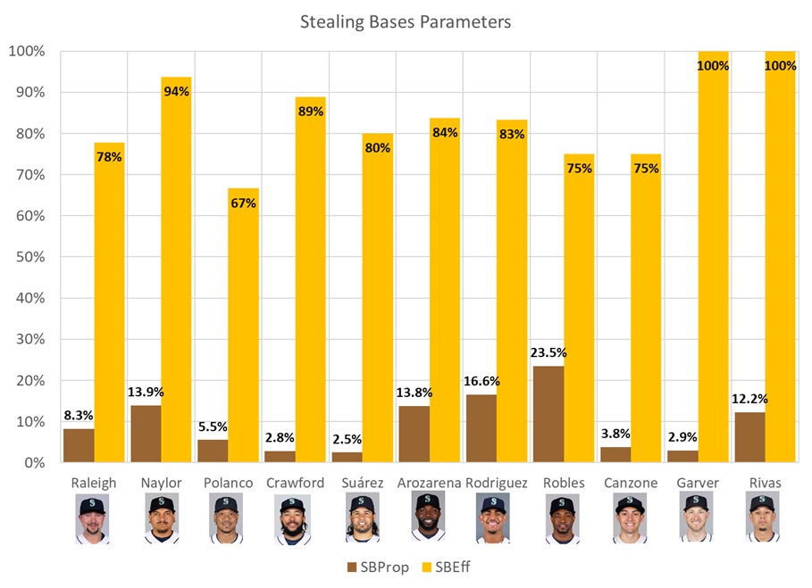
The chart above shows the stealing process probabilities. The brown bar shows the propensity probability while the yellow bar shows the efficiency. For instance, Suárez was successful 80% of the times trying to steal, but clearly, he doesn’t try a steal very often (only 2.5% of the times where a base was available to steal). On the other hand, Robles was the player that tried to steal more often with a 23.5% propensity rate, but was not the most successful at it (only 75%). Rodríguez and Arozarena contributed to the team in the running game as they tried many times (16.6% and 13.8% of their chances) with good success at it (83% and 84% respectively). Surprisingly Naylor which isn’t a fast player, was successful on a whopping 94% of the steal attempts he had.
2,000 different games were simulated using the “naïve” lineup consisting of an order of the players by position played, the following chart summarizes the distribution of runs scored per game:
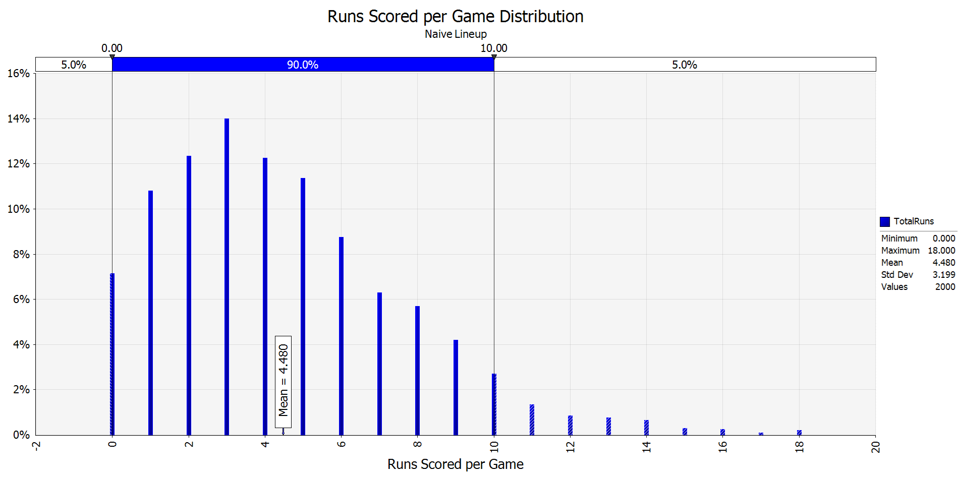
The chart shows the stochastic process, in which a random number of runs are scored per game even using the same naïve lineup in all 2,000 games. In some games, the lineup scores 3 runs, which is the most likely outcome (highest bar), but even 18 runs are possible although with a very low probability. The mean runs scored per game (mrsg) is equal to 4.48, which is the expected number of runs this lineup will score over a long run, this would extrapolate to a total of 726 runs scored over a 162 game-season. As a comparison, the Mariners scored a total of 766 runs during the actual 2025 season, so this shows that the estimation made by our model is not that far off from the actual mrsg of 4.728 (766 / 162) scored by the 2025 Mariners.
Optimization
The main goal of this project is to optimize the lineup that the manager can use. Even though players are not strat-o-matic cards, and perform robotically mimicking their stats, and it is well known that some player perform better on different lineup spots depending on their psychology, we can use this model to try to optimize the lineup at least based on what statistics tell.
To optimize the lineup, we can test different combinations of lineups until “the best” one is achieved. Best will be defined in terms of maximizing the mean runs scored per game (mrsg) of the lineup. But trying all combinations would be a tedious and time-consuming process (remember there are almost 40 million different possible lineup combinations). A more effective alternative would be the use of genetic algorithms.
A genetic algorithm is a heuristic search that mimics the natural evolution process. This algorithm is routinely used to find optimization solutions, which belong to a class of algorithms inspired by natural evolution using concepts such as heritage, mutation, selection and mixing.
In a genetic algorithm a chain population (called chromosomes) that carry coded possible candidates for solutions (called individuals or phenotypes) evolve to find better solutions. Traditionally solutions are represented as a binary chain of 0 and 1. Evolution usually starts with a population of individuals randomly generated as a first generation. For each new generation, the aptitude of each individual is evaluated and multiple individuals are selected stochastically (based upon their aptitude) and subsequently modified (mixed or randomly mutated) to form a new population. The new population is used for the next iteration. Normally the algorithm ends when a determined number of generations have been produced or when a certain level of aptitude in the population has been achieved. If the algorithm ends because of the first criteria the “best solution” may not have been found.

Genetic algorithm example of chromosome generation.
Hence, the genetic algorithm was applied to the run scoring simulation model with the goal of optimizing the lineup. The variable to optimize is stochastic, because it is the average of the iterations of the stochastic process. In other words, the algorithm will search to maximize the mean runs scored per game (mrsg) of different lineups in a smart way.
RiskOptimizer from @Risk includes different solution algorithms, through which the adjustable cells get modified. In this case, the adjustable cells are the 11 lineup spots, although only the first 9 will play the game, and the solution method proposed is “order” so in each solution a different order of the 11 possible players is tried.

Lineup optimization process
Optimization results
The optimization process was let run for 0:47 minutes and 1,267 trials and the following chart summarizes the progress of the process:

Optimization progress chart
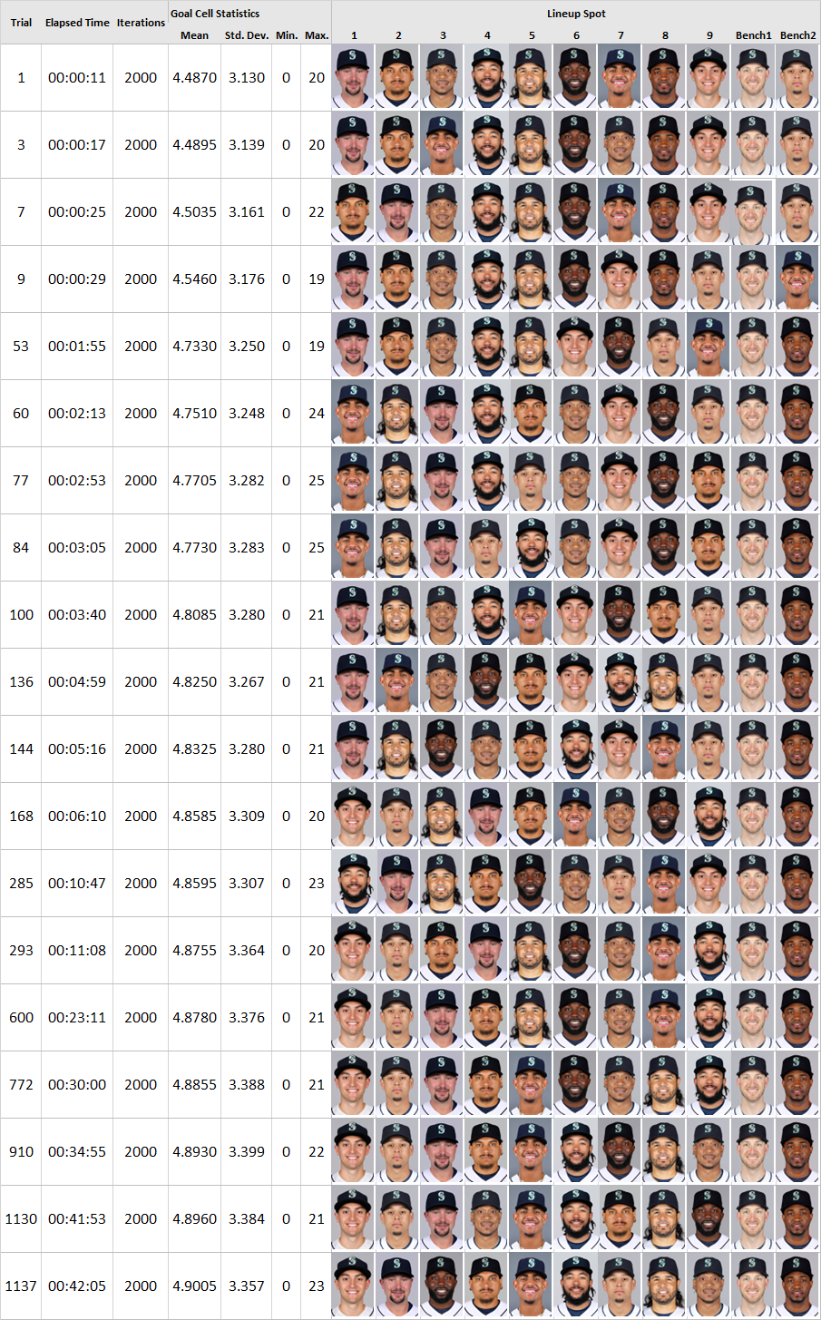
2025 Seattle Mariners Optimization process
From the naïve lineup the process found a better solution in trial #3 in which Polanco and Rodríguez switched spots and the mrsg = 4.4895. This process kept finding better solutions in trials 7, 9, 53, 60, etc. and even though the “best” lineup was found on trial # 1,137, it can continue for a longer time, and thus this “best” lineup is not guaranteed to be the actual best. A better one can still be achieved if the process is run for a longer time.
An analysis of the final rows show that Canzone is a better fit for the leadoff spot because the last 6 solutions have him as the #1 spot, while it is also clear that Garver and Robles are better off to be left on the bench (Garver played the role of the backup catcher for most of the season so this makes sense).
The “best” lineup that the model found was this one:
1. Canzone
2. Raleigh
3. Arozarena
4. Naylor
5. Rodríguez
6. Crawford
7. Rivas
8. Suárez
9. Polanco
This lineup scores an average of 4.9005 runs per game, which is quite an improvement over the 4.48 mrsg of the naïve lineup, and it would translate to 794 runs scored for a whole season. Keep in mind that the actual number of runs scored by the 2025 Mariners was 766, so this lineup would, on paper, be better than the actual 2025 Mariners.
Although this lineup might not seem like a “good” lineup to the casual fan, because Canzone never batted leadoff and Polanco, the ALDS hero is batting 9th, this is the “best” lineup found after almost an hour of the model running. Keep in mind that the model is using 2025 regular season stats for each player, and Canzone had a very good slash line of AVG, OBP and SLG of: .300 / .358 / .481 over 268 plate appearance. Short memory bias can make us think that other players might be a better fit. For instance, Polanco had this slash lines:
Regular Season: .265 / .326 / .495
Post Season: .208 / .269 / .417
But let’s not forget that the regular season stats are based on a sample size of 524 plate appearances, while the post season stats are based on 52 plate appearances (roughly 10% of the regular season ones), thus making the probabilities estimated using regular season stats more reliable.